[10]:
import numpy as np
import matplotlib.pyplot as plt

from scipy.stats import mode

from muldoon.met_timeseries import PressureTimeseries
from muldoon.utils import *
from muldoon.read_data import *
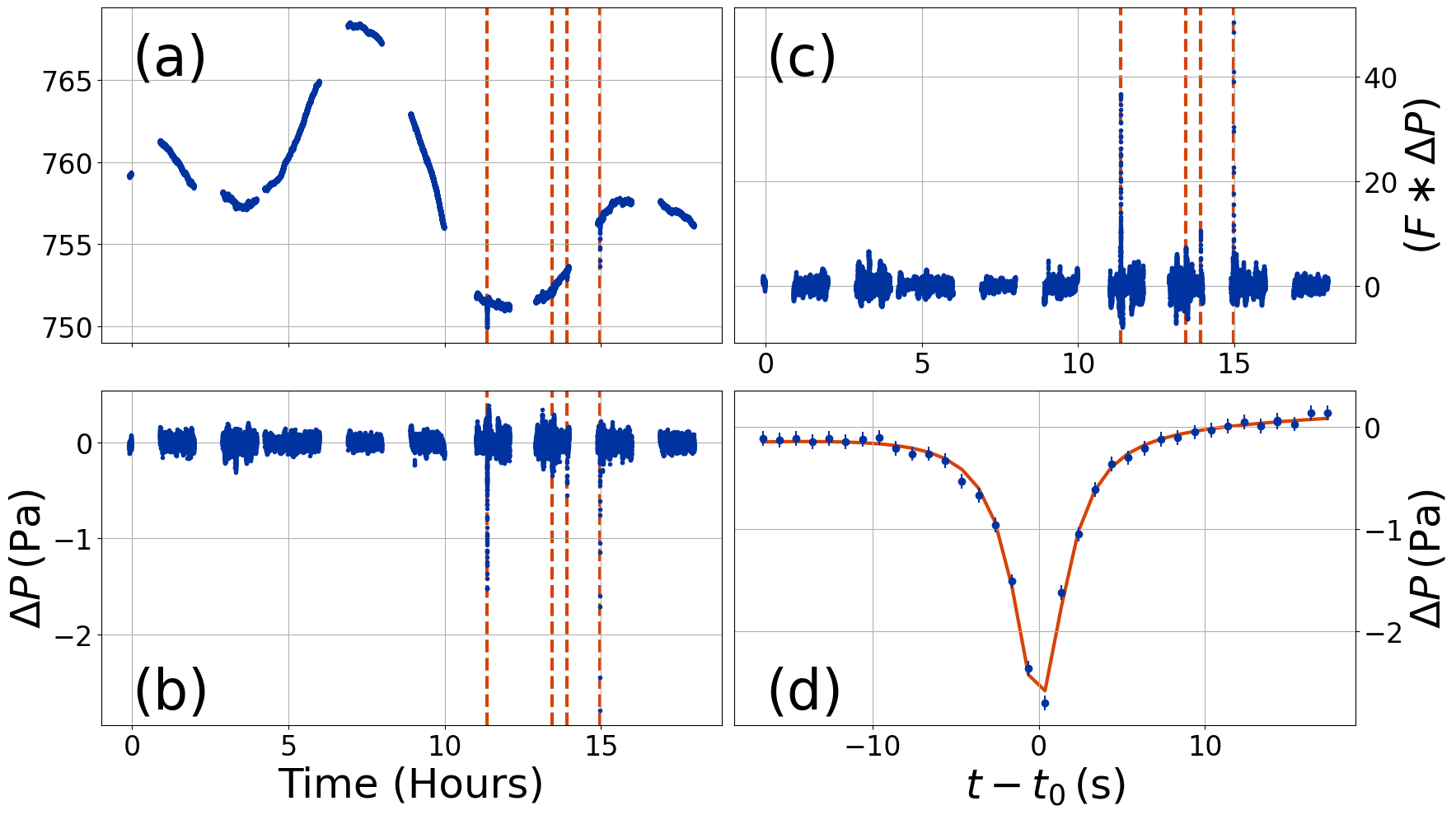
[3]:
# Read in data file
filename = "./WE__0089___________DER_PS__________________P01.CSV"
time, pressure = read_Perseverance_PS_data(filename)
# plt.scatter(time, pressure)

times, pressures = break_at_gaps(time, pressure)

fig = plt.figure(figsize=(10, 10))
ax = fig.add_subplot(111)

for i in range(len(times)):
#     plt.axvline(time[0:-1][gaps][i])
    ax.scatter(times[i], pressures[i], marker='.')
ax.grid(True)
Processing file: ./WE__0089___________DER_PS__________________P01.CSV
===================================================================
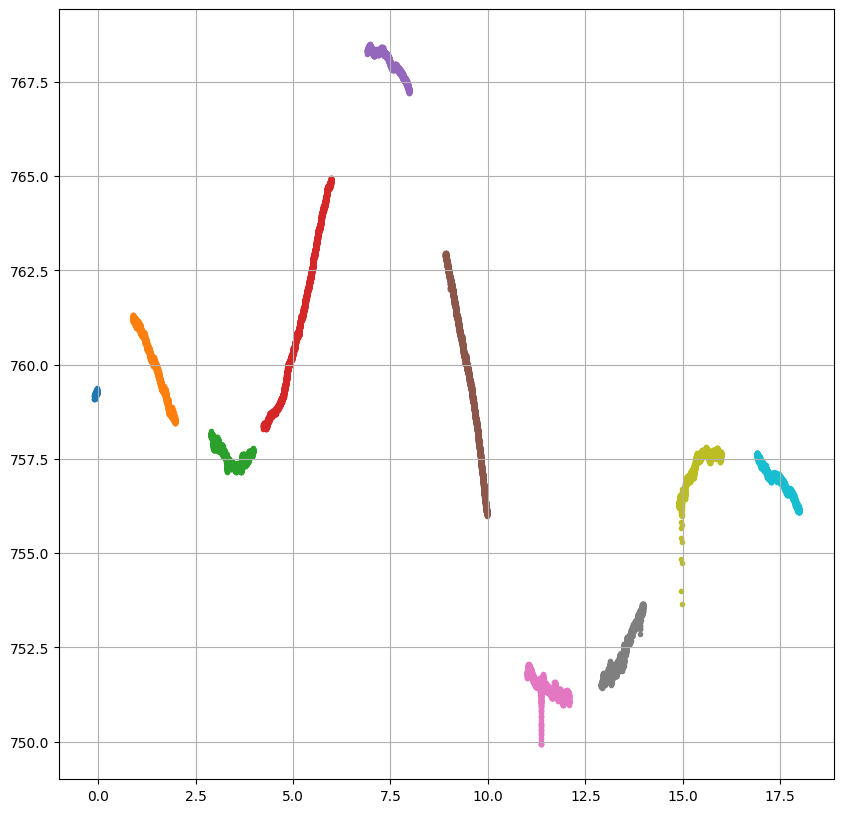
[11]:
# Detrend

mt = PressureTimeseries(time, pressure)

window_size = 500./3600 # window size is 500 seconds
mt.detrend_timeseries_boxcar(window_size)

fig = plt.figure(figsize=(10, 10))
ax = fig.add_subplot(111)
ax.scatter(mt.time, mt.detrended_data, marker='.')
ax.grid(True)
[12]:
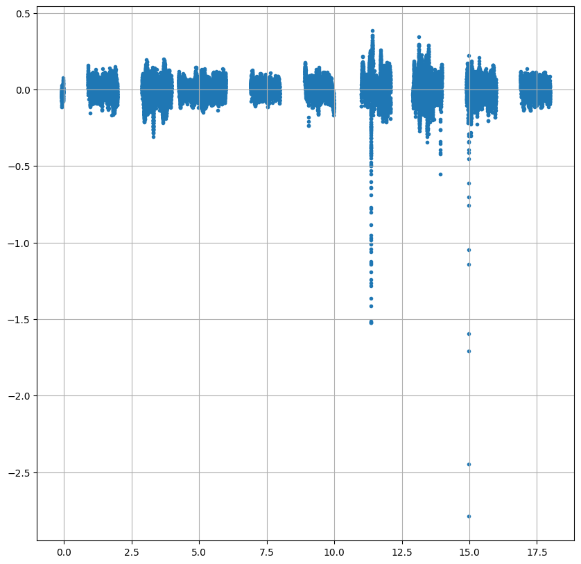
# Detect vortex signals
matched_filter_width = 2.*mt.sampling
matched_filter_depth = 1./np.pi
distance_between_peaks = 30
detection_threshold = 7.

conv = mt.apply_lorentzian_matched_filter(matched_filter_width, matched_filter_depth)
vortices = mt.find_vortices(detection_threshold=detection_threshold, distance=distance_between_peaks)

fig = plt.figure(figsize=(10, 10))
ax = fig.add_subplot(111)

ax.plot(mt.time, mt.convolution, ls='', marker='.')
ax.axhline(detection_threshold)

for i in range(len(mt.peak_indices)):
    ax.axvline(mt.time[mt.peak_indices[i]], color="orange", zorder=-1)
[13]:
mt.fit_all_vortices(filepath="./WE__0089");
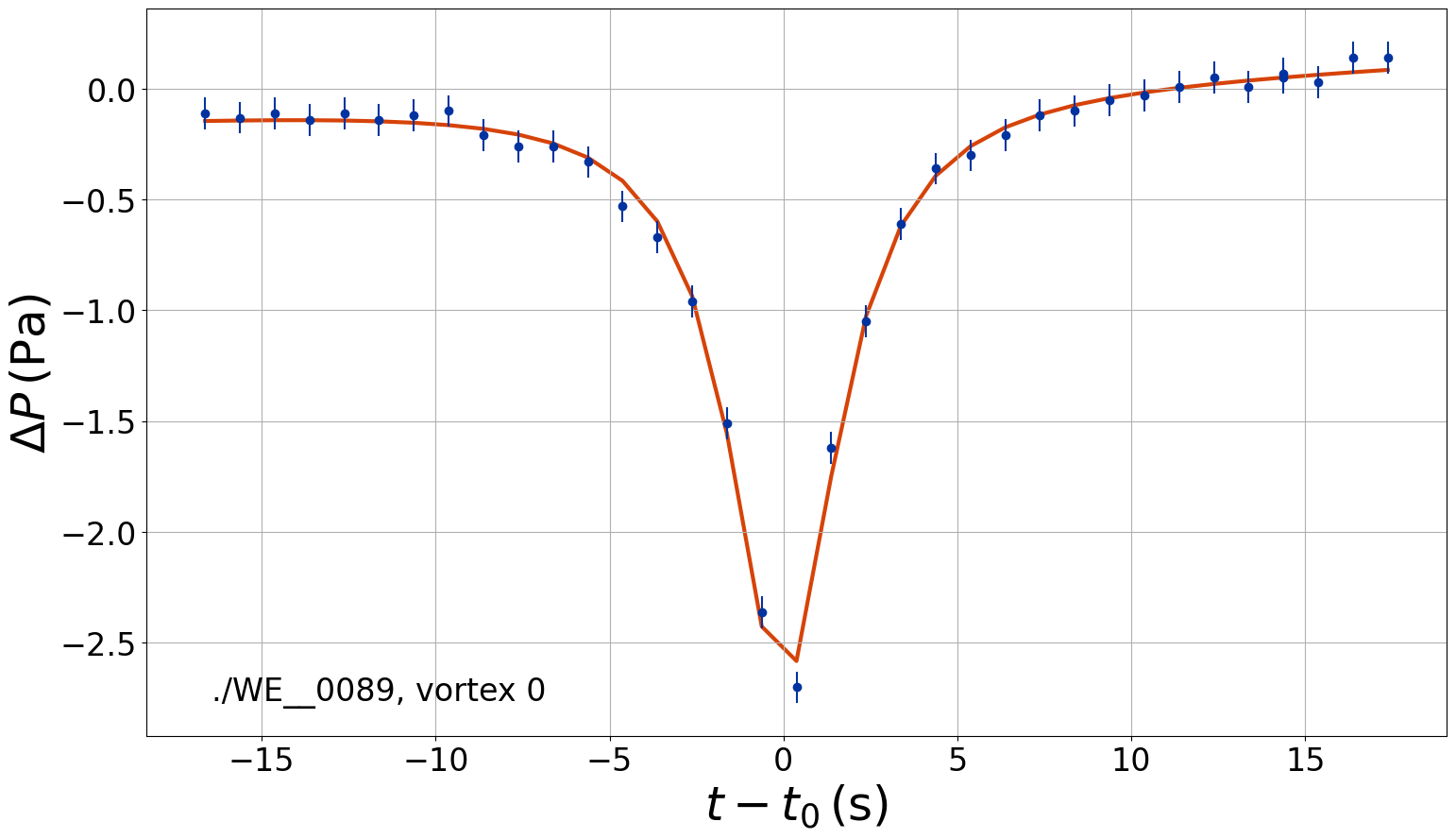
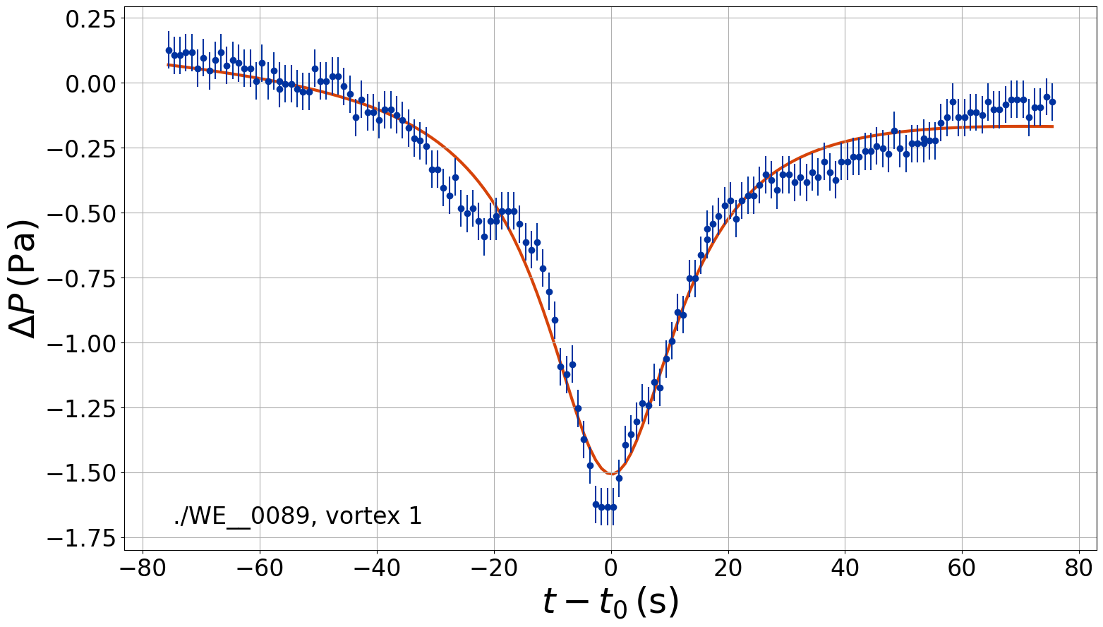

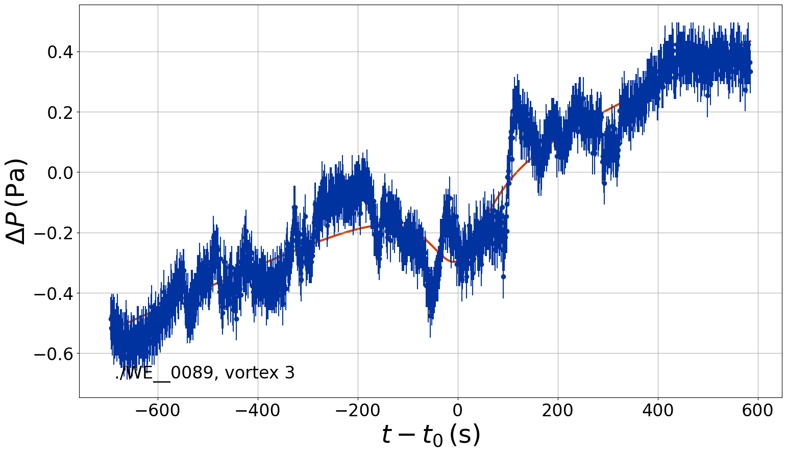
[14]:
# Make final conditioned data figure
mt.make_conditioned_data_figure(which_vortex=0);
plt.tight_layout()