Using Muldoon

Here are some examples for how to use some of the functionality of Muldoon.

%matplotlib inline
%config InlineBackend.figure_format='retina'
%load_ext autoreload
%autoreload 2

import numpy as np
import matplotlib.pyplot as plt

from numpy.random import normal

from scipy.stats import median_abs_deviation as mad

from muldoon.met_timeseries import MetTimeseries, PressureTimeseries, TemperatureTimeseries
from muldoon.utils import modified_lorentzian, fit_vortex, write_out_plot_data
from muldoon.read_data import *

The autoreload extension is already loaded. To reload it, use:
  %reload_ext autoreload

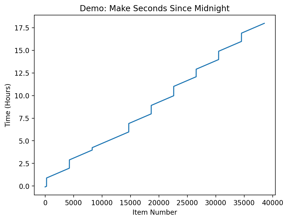
Make Seconds Since Midnight Plot

filename="WE__0089___________DER_PS__________________P01.CSV"
time = make_seconds_since_midnight(filename)
plt.title("Demo: Make Seconds Since Midnight")
plt.xlabel("Item Number")
plt.ylabel("Time (Hours)")
plt.plot(time)

Processing file: WE__0089___________DER_PS__________________P01.CSV
===================================================================

[<matplotlib.lines.Line2D at 0x7fb5999a9bd0>]

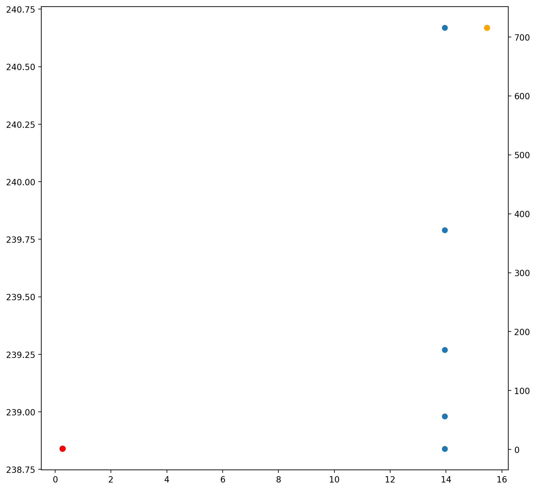
Read Data Function

fig = plt.figure(figsize=(10,10))
ax = fig.add_subplot(111)
ax2 = ax.twinx()

# Read Temperature (ATS) Data
ATSfilename='https://pds-atmospheres.nmsu.edu/PDS/data/PDS4/Mars2020/mars2020_meda/data_calibrated_env/sol_0000_0089/sol_0010/WE__0010___________CAL_ATS_________________P01.xml'
temperature_time, temperature = read_Perseverance_ATS_data(ATSfilename, which_ATS=1, end=5)
ax.scatter(temperature_time, temperature)

# Read Pressure (PS) Data
PSfilename="https://pds-atmospheres.nmsu.edu/PDS/data/PDS4/Mars2020/mars2020_meda/data_derived_env/sol_0000_0089/sol_0001/WE__0001___________DER_PS__________________P02.xml"
pressure_time, pressure = read_Perseverance_PS_data(PSfilename, end=5)
ax2.scatter(pressure_time, pressure, color='orange')

# Read Wind (WS) Data
WSfilename='https://pds-atmospheres.nmsu.edu/PDS/data/PDS4/Mars2020/mars2020_meda/data_derived_env/sol_0180_0299/sol_0190/WE__0190___________DER_WS__________________P02.xml'
wind_time, wind = read_Perseverance_WS_data(WSfilename, end=5)
ax2.scatter(wind_time, wind, color='red')

Processing label: https://pds-atmospheres.nmsu.edu/PDS/data/PDS4/Mars2020/mars2020_meda/data_calibrated_env/sol_0000_0089/sol_0010/WE__0010___________CAL_ATS_________________P01.xml
Found a Header structure: HEADER
Found a Table_Delimited structure: TABLE
===================================================================
Processing label: https://pds-atmospheres.nmsu.edu/PDS/data/PDS4/Mars2020/mars2020_meda/data_derived_env/sol_0000_0089/sol_0001/WE__0001___________DER_PS__________________P02.xml
Found a Header structure: HEADER
Found a Table_Delimited structure: TABLE
===================================================================
Processing label: https://pds-atmospheres.nmsu.edu/PDS/data/PDS4/Mars2020/mars2020_meda/data_derived_env/sol_0180_0299/sol_0190/WE__0190___________DER_WS__________________P02.xml
Found a Header structure: HEADER
Found a Table_Delimited structure: TABLE
===================================================================

<matplotlib.collections.PathCollection at 0x7fb598598400>

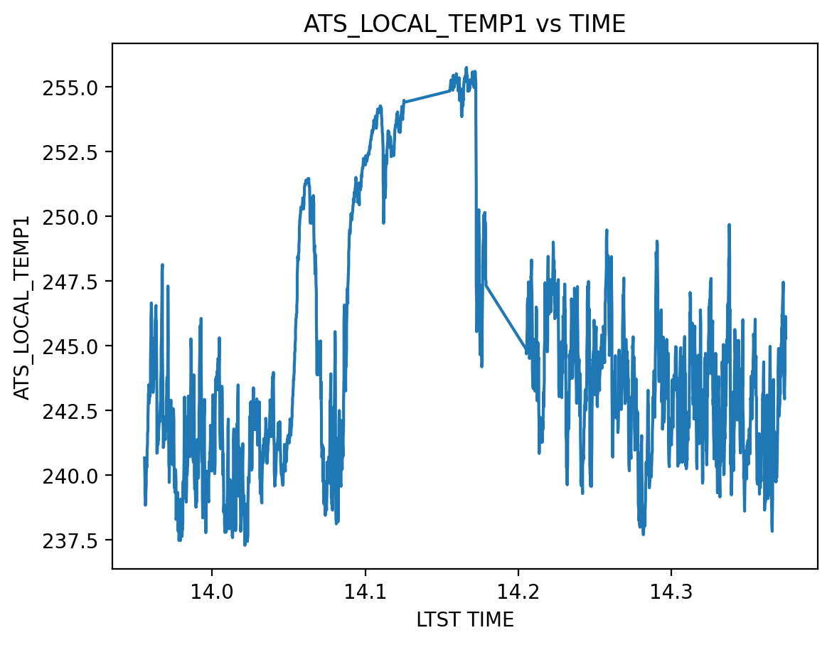
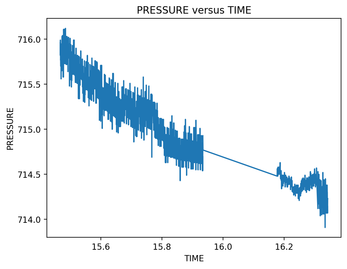
Plot Data Function

---

# Reads and plots Temperature vs Time
plot_Perseverance_ATS_data(ATSfilename)

# Reads and plots Pressure vs Time
plot_Perseverance_PS_data(PSfilename)

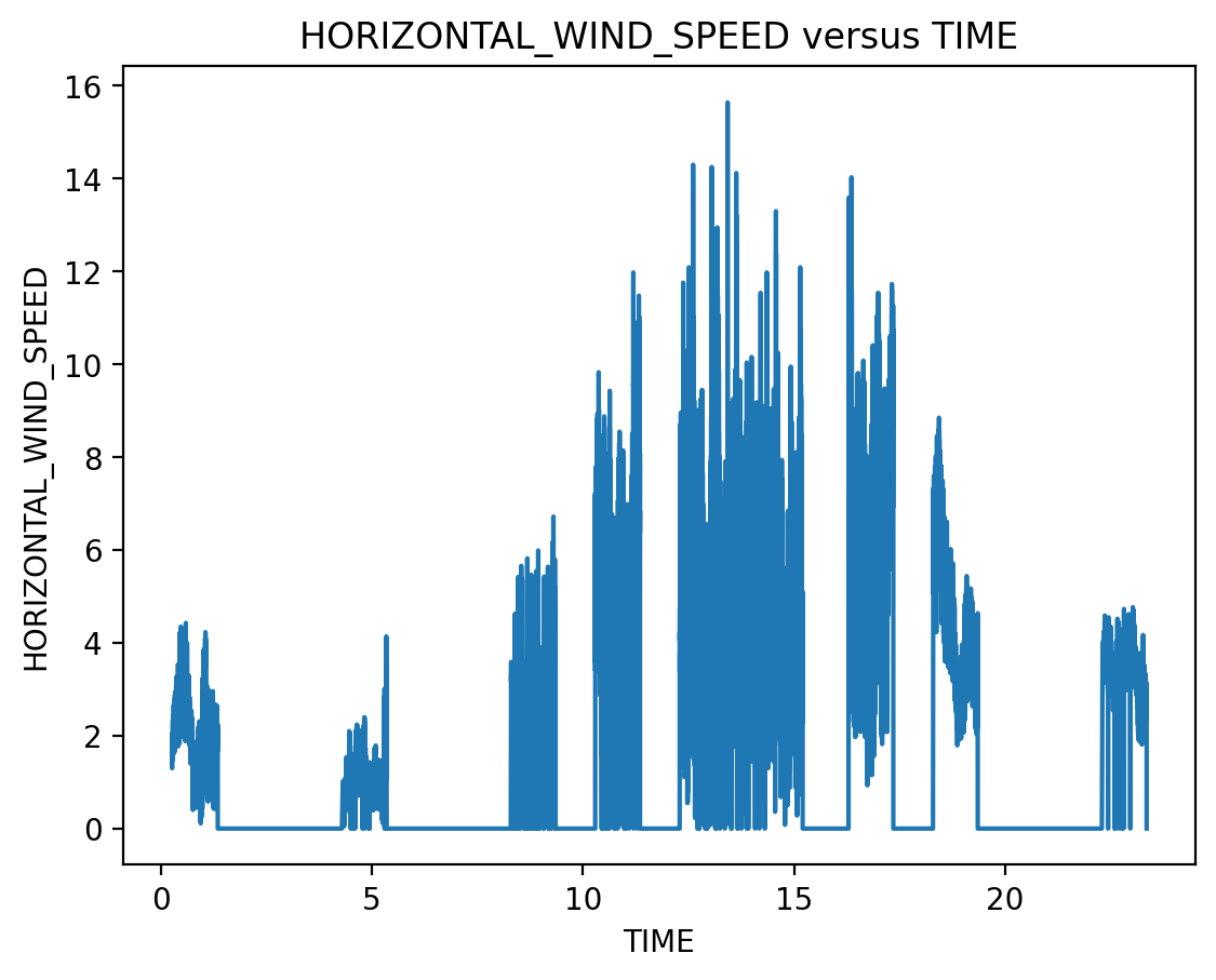
# Reads and plots Wind vs Time
plot_Perseverance_WS_data(WSfilename)

Processing label: https://pds-atmospheres.nmsu.edu/PDS/data/PDS4/Mars2020/mars2020_meda/data_calibrated_env/sol_0000_0089/sol_0010/WE__0010___________CAL_ATS_________________P01.xml
Found a Header structure: HEADER
Found a Table_Delimited structure: TABLE
===================================================================

Processing label: https://pds-atmospheres.nmsu.edu/PDS/data/PDS4/Mars2020/mars2020_meda/data_derived_env/sol_0000_0089/sol_0001/WE__0001___________DER_PS__________________P02.xml
Found a Header structure: HEADER
Found a Table_Delimited structure: TABLE
===================================================================

Processing label: https://pds-atmospheres.nmsu.edu/PDS/data/PDS4/Mars2020/mars2020_meda/data_derived_env/sol_0180_0299/sol_0190/WE__0190___________DER_WS__________________P02.xml
Found a Header structure: HEADER
Found a Table_Delimited structure: TABLE
===================================================================

Testing Pressure Time Series

---

# Create time-series
time = np.linspace(-10, 10, 1000)
baseline = 0.
slope = 1.
t0 = 0.
DeltaP = 1.
Gamma = 0.5

right_answer = np.array([baseline, slope, t0, DeltaP, Gamma])

profile = modified_lorentzian(time, baseline, slope, t0, DeltaP, Gamma) + normal(scale=slope/20., size=len(time))
mt = PressureTimeseries(time, profile)

Detrended Data Graph Demonstration

---

# Detrend
window_size = Gamma
detrended_pressure = mt.detrend_timeseries_boxcar(window_size)
print(np.std(mt.detrended_data))
print(np.isclose(np.std(mt.detrended_data), 0.1, atol=0.1))

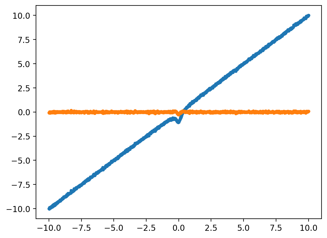
plt.scatter(mt.time, mt.data, marker='.')
plt.scatter(mt.time, mt.detrended_data, marker='.')

0.05237482150437607
True

<matplotlib.collections.PathCollection at 0x7fb598802b30>

# Test time-series write-out
write_str = write_out_plot_data(mt.time, mt.data, yerr=np.std(mt.data)*np.ones_like(mt.data),
                                x_label="Time", y_label="Pressure", test_mode=True)

Plot Profiling Demonstration

---

# plt.plot(mt.time, profile)
conv = mt.apply_lorentzian_matched_filter(2.*mt.sampling, 1./np.pi)
mx_ind = np.argmax(mt.convolution)

print(mt.convolution[mx_ind], np.abs(mt.time[mx_ind]), 2.*mt.sampling)
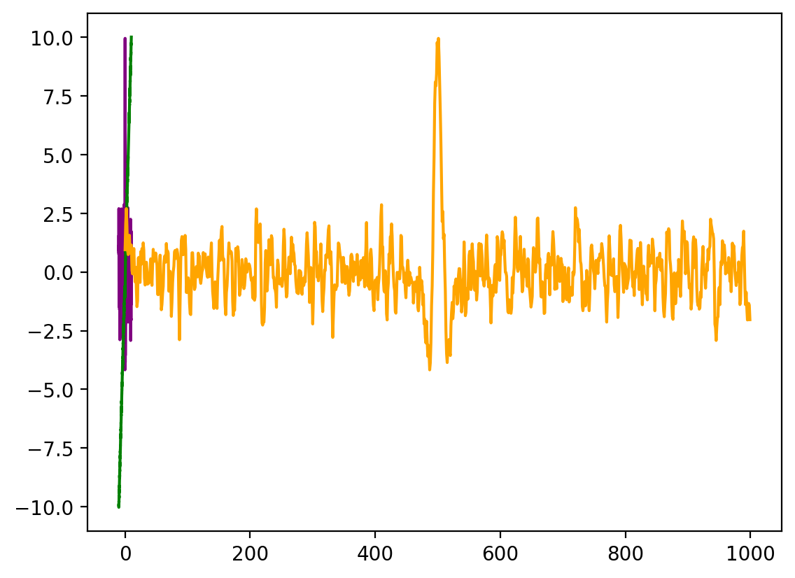
plt.plot(mt.time, mt.convolution, color="purple")
plt.plot(mt.time, profile, color="green")
plt.plot(mt.convolution, color="orange")
# Make sure convolution returns a strong peak at the right time
print((np.abs(mt.time[mx_ind])))

9.960900121027885 0.03003003003003002 0.040040040040040026
0.03003003003003002

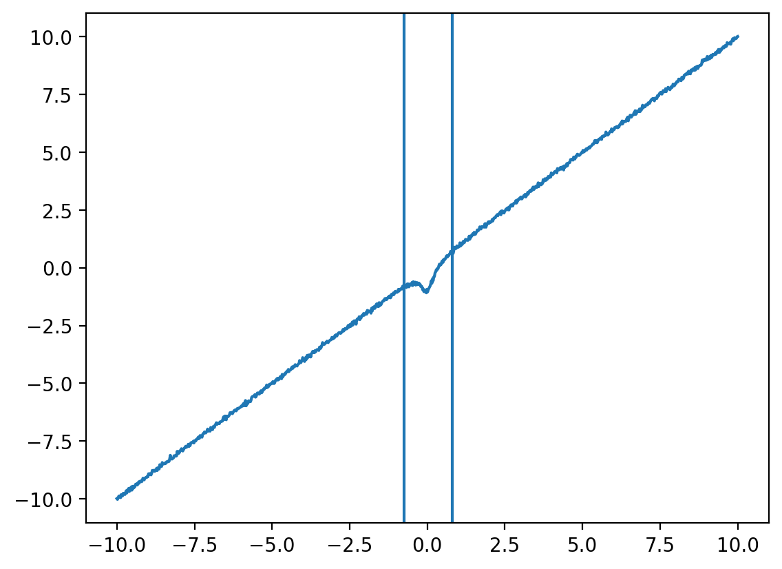
Find Vortices Demonstration

---

vortices = mt.find_vortices(detection_threshold=2)
plt.plot(mt.convolution)
plt.axvline(mt.peak_indices[0] - 3.*mt.peak_widths[0])
plt.axvline(mt.peak_indices[0] + 3.*mt.peak_widths[0])

# Make sure the max peak in the convolution is the right one
assert(mt.time[mt.peak_indices[0]] < Gamma)

# Test find_vortices
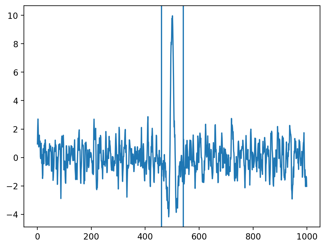
vortices = mt.find_vortices(detection_threshold=7)
plt.plot(mt.time, mt.data)
plt.axvline(mt.time[mt.peak_indices[0] - 3*int(mt.peak_widths[0])])
plt.axvline(mt.time[mt.peak_indices[0] + 3*int(mt.peak_widths[0])])

<matplotlib.lines.Line2D at 0x7fb598ae4250>

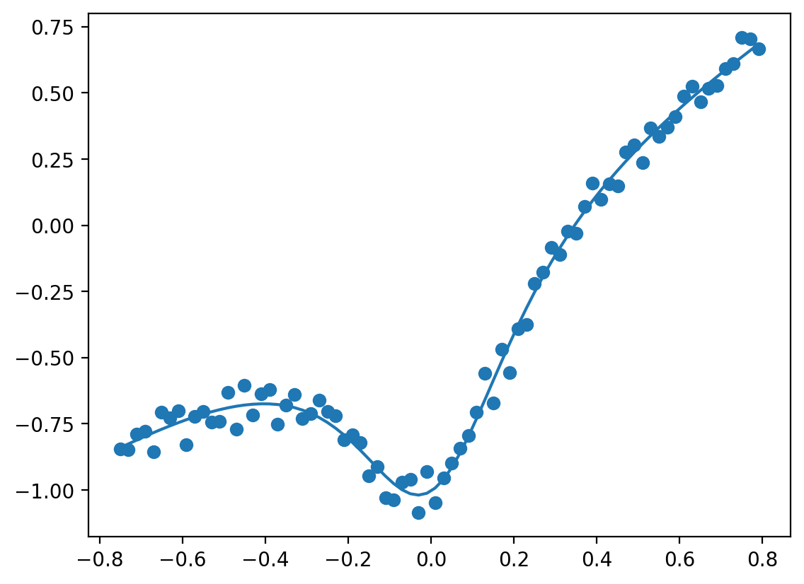
Vortex Fit Demonstration

---

plt.scatter(vortices[0]["time"], vortices[0]["data"])

# Test vortex fit
old_popt, old_unc = fit_vortex(vortices[0], [0., 1., 0., 1., 0.01],
                          [[-1, -1, np.min(vortices[0]["time"]), 0, 0],
                           [1, 1, np.max(vortices[0]["time"]), 2, 1]], sigma=vortices[0]["scatter"])
assert(np.max(np.abs(old_popt - right_answer)/old_unc) < 3.)

plt.plot(vortices[0]["time"], modified_lorentzian(vortices[0]["time"], *old_popt))

[<matplotlib.lines.Line2D at 0x7fb596342650>]

init_params = mt._determine_init_params(vortices[0])
bounds = mt._determine_bounds(vortices[0], init_params)
popt, unc = fit_vortex(vortices[0], init_params, bounds, sigma=vortices[0]["scatter"])
assert(np.max(np.abs(popt - right_answer)/unc) < 3.)

print(np.max(np.abs(popt - right_answer)/unc))

1.223916561695807

Fit All Vortices Demonstration

---

# Test fit all vortices

# Create time-series
time = np.linspace(-10, 10, 1000)
baseline = 0.
slope = 1.
t0 = 0.
DeltaP = 1.
Gamma = 0.5

right_answer = np.array([baseline, slope, t0, DeltaP, Gamma])

profile = modified_lorentzian(time, baseline, slope, t0, DeltaP, Gamma) + normal(scale=slope/20., size=len(time))
mt = PressureTimeseries(time, profile)
window_size = Gamma
detrended_pressure = mt.detrend_timeseries_boxcar(window_size)

conv = mt.apply_lorentzian_matched_filter(2.*mt.sampling, 1./np.pi)
vortices = mt.find_vortices(detection_threshold=7)

popts, uncs = mt.fit_all_vortices()
print(np.max(np.abs(popts[0] - right_answer)/uncs[0]))
assert(np.max(np.abs(popts[0] - right_answer)/uncs[0]) < 5.)

1.1426068795027213

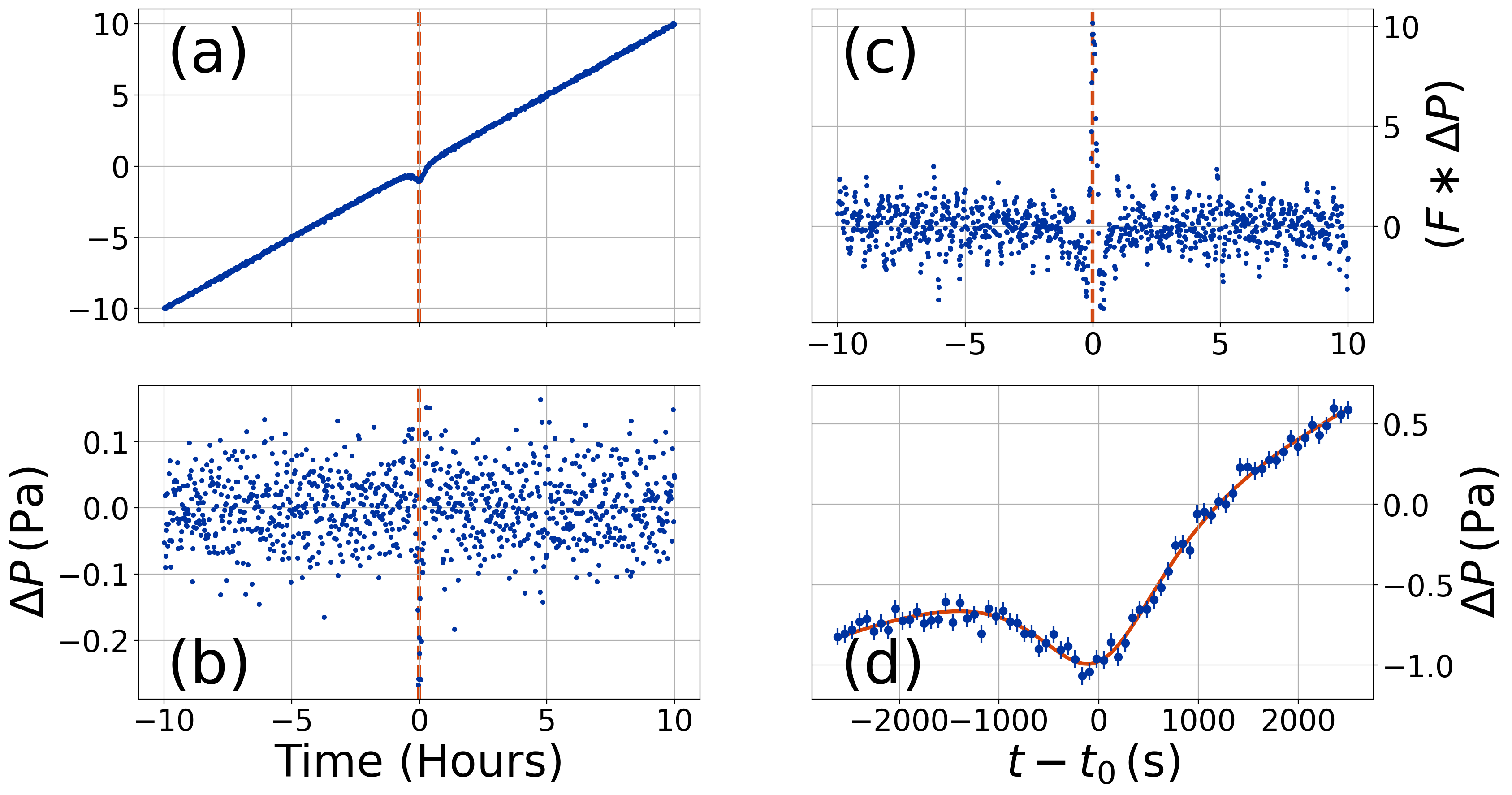
Condition Fit/Per-Panel Write-Out Demonstration

---

# Make plot showing how the data are conditioned and write out the data in each panel
mt.make_conditioned_data_figure(write_filename="./test_");

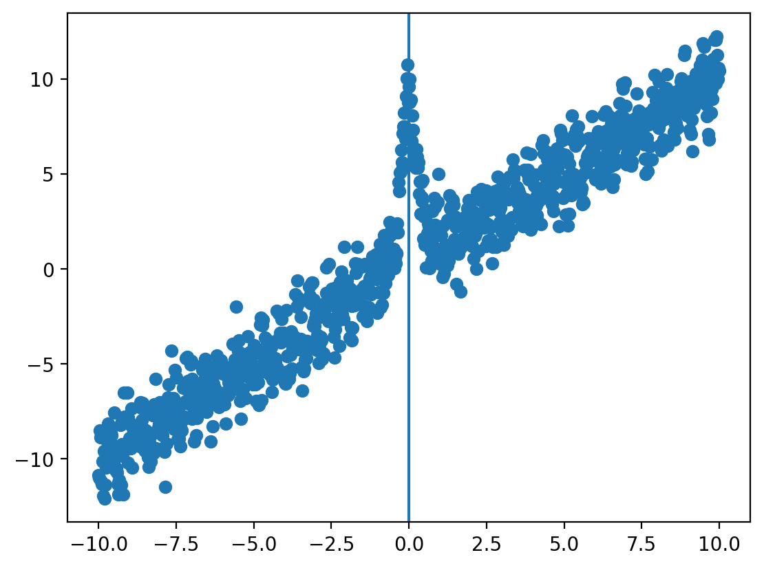
Further Time-Series Demonstration (With Added Noise/Interference to Data)

---

# Create time-series
time = np.linspace(-10, 10, 1000)
baseline = 0.
slope = 1.
t0 = 0.
DeltaP = 1.
Gamma = 0.5

DeltaT = -10.

right_answer = np.array([baseline, slope, t0, DeltaP, Gamma])
temp_right_answer = np.array([baseline, slope, t0, DeltaT, Gamma])

profile = modified_lorentzian(time, baseline, slope, t0, DeltaP, Gamma) + normal(scale=slope/20., size=len(time))
mt = PressureTimeseries(time, profile)

# Add in some nasty sine wave action
red_noise_period = Gamma
temp_profile = modified_lorentzian(time, *temp_right_answer) +\
    normal(scale=slope, size=len(time)) + DeltaT/10.*np.sin(2*np.pi/red_noise_period*time)
tt = TemperatureTimeseries(time, temp_profile,
                           popts=[right_answer],
                           uncs=[np.array([0, 0, 0, 0, 0])])
plt.scatter(tt.time, tt.data)

plt.axvline(tt.popts[0][2])

<matplotlib.lines.Line2D at 0x7fb599905540>

Retrieve Vortices Demonstration

---

tt.retrieve_vortices()
plt.scatter(tt.vortices[0]["time"], tt.vortices[0]["data"])
print(len(tt.vortices[0]["time"]))

150

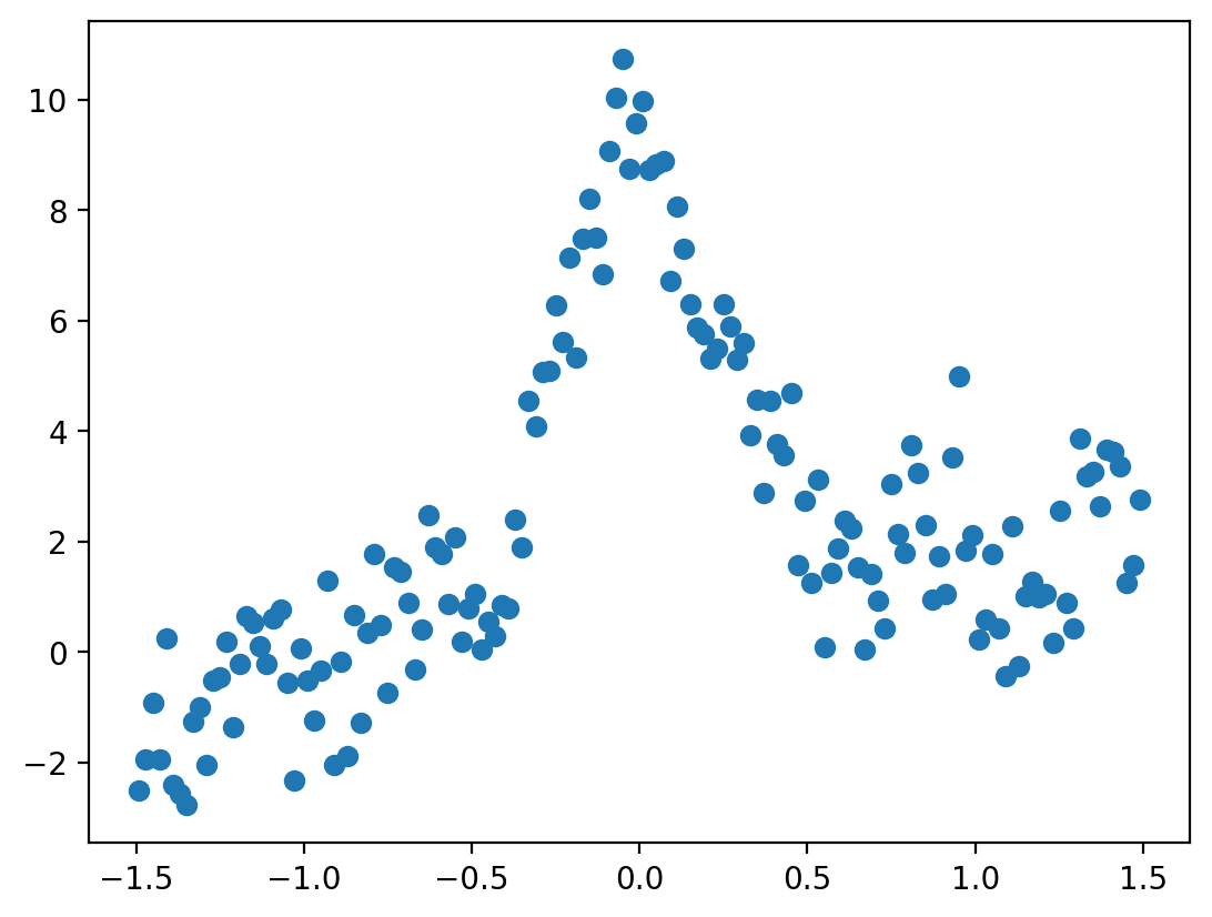
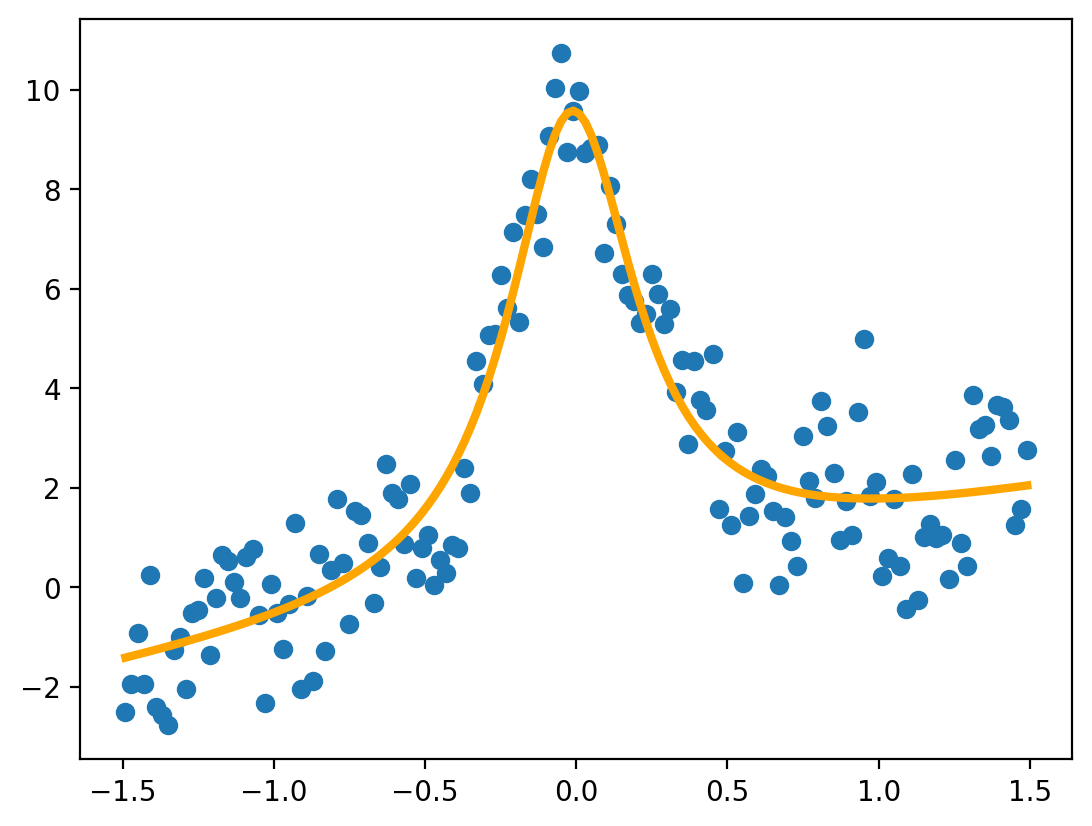
Vortex Normal Linear Regression Demonstration

---

# Fit vortex using normal linear regression
# baseline, slope, t0, DeltaT, Gamma
temp_baseline = np.mean(tt.vortices[0]["data"])
temp_avg_slope = (tt.vortices[0]["data"][-1] - tt.vortices[0]["data"][0])/\
    (tt.vortices[0]["time"][-1] - tt.vortices[0]["time"][0])
max_excursion = -np.abs(np.max(tt.vortices[0]["data"]) - np.min(tt.vortices[0]["data"]))

sigma = mad(tt.vortices[0]["data"])

init_params = [temp_baseline, temp_avg_slope, t0, max_excursion, Gamma]
bounds = [[np.min(tt.vortices[0]["data"]), -3.*np.abs(temp_avg_slope), np.min(tt.vortices[0]["time"]),
           -3.*np.abs(max_excursion), 0.],
          [np.max(tt.vortices[0]["data"]),  3.*np.abs(temp_avg_slope), np.max(tt.vortices[0]["time"]),
            0., 3.*Gamma]]

popt, unc = fit_vortex(tt.vortices[0], init_params, bounds)
# print(popt)
# print(unc)
# print(temp_right_answer)

plt.scatter(tt.vortices[0]["time"], tt.vortices[0]["data"])
plt.plot(tt.vortices[0]["time"], modified_lorentzian(tt.vortices[0]["time"], *popt), lw=3, color='orange')

[<matplotlib.lines.Line2D at 0x7fb5988aa1a0>]

# Fit vortex using Gaussian processes - https://george.readthedocs.io/en/latest/tutorials/model/

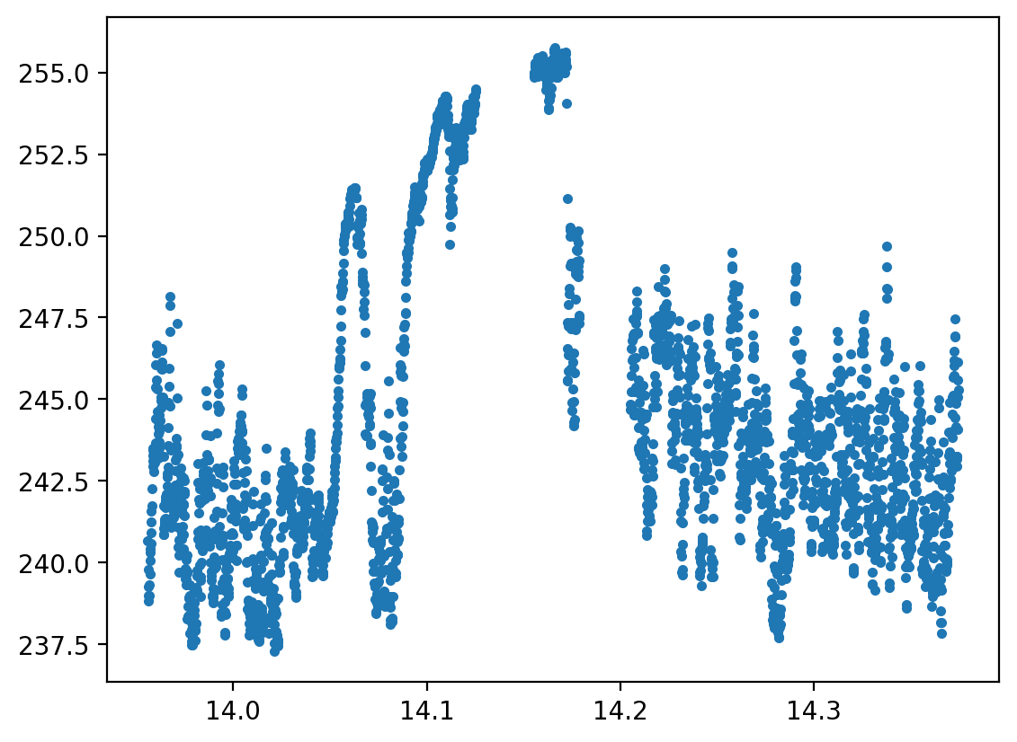
Temperature Time Series Demonstration

---

time, temperature = read_Perseverance_ATS_data(ATSfilename, which_ATS=1)
tt = TemperatureTimeseries(time, temperature)
plt.scatter(tt.time, tt.data, marker='.')

Processing label: https://pds-atmospheres.nmsu.edu/PDS/data/PDS4/Mars2020/mars2020_meda/data_calibrated_env/sol_0000_0089/sol_0010/WE__0010___________CAL_ATS_________________P01.xml
Found a Header structure: HEADER
Found a Table_Delimited structure: TABLE
===================================================================

<matplotlib.collections.PathCollection at 0x7fb5987e5000>

###                     Currently experience div-by-zero error                     ###

# Detrend
# window_size = 1. # 1 hour
# detrended_temperature = tt.detrend_timeseries_boxcar(window_size)
# plt.scatter(tt.time, tt.detrended_data, marker='.')